RNN
이번엔 순환신경망, RNN에 대한 내용이다.
여기서는 순차데이터를 다루는데 데이터들이 독립적이지 않고 서로 연관된 데이터(sequential data)에 관한 내용이다. 그 중에서도 일정 시간 간격으로 배치된 데이터를 시계열(time series) 데이터라고 한다. 그리고 순차 데이터를 처리하는 각 단계는 Time step이라고 부른다.
예를 들면 어떠한 문장은 앞 단어와 뒷 단어가 연관성을 가지는 순차 데이터라 할 수 있다.
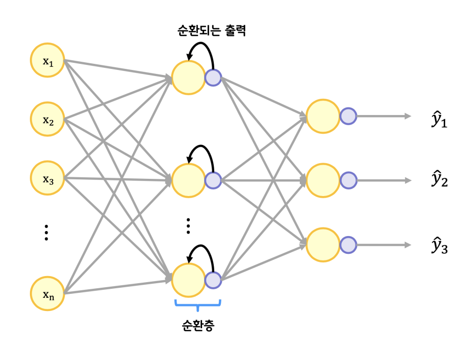
이런 순차데이터는 순환층을 이용하여 처리하는데 출력을 다시 입력에 넣어서 순환시키는 구조이다.
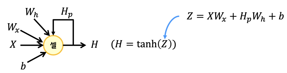
순환구조에는 지난번에 소개했던 하이퍼볼릭탄젠트 함수를 사용한다. 그리고 위와 같은 신경망 중 순환신경망을 셀이라고 부른다. 단위를 나눈다는 것은 추상화해서 감추겠다는 것이겠지. 늘 그렇듯.
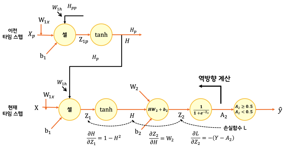
시계열 데이터이므로 역전파도 시간을 거스르는데 이 방식을 BPTT(Backpropagation Through Time)라고 부른다. 특정시간을 정해서 시간을 거슬러 역전파하는 방식은 TBPTT(Truncated-Backpropagation Through Time)이라 한다. 코드로 살펴보면 아래와 같다.
class RecurrentNetwork:

    def __init__(self, n_cells=10, batch_size=32, learning_rate=0.1):
        self.n_cells = n_cells     # 셀 개수
        self.batch_size = batch_size     # 배치 크기
        self.w1h = None            # 은닉 상태에 대한 가중치
        self.w1x = None            # 입력에 대한 가중치
        self.b1 = None             # 순환층의 절편
        self.w2 = None             # 출력층의 가중치
        self.b2 = None             # 출력층의 절편
        self.h = None              # 순환층의 활성화 출력
        self.losses = []           # 훈련 손실
        self.val_losses = []       # 검증 손실
        self.lr = learning_rate    # 학습률

    def forpass(self, x):
        self.h = [np.zeros((x.shape[0], self.n_cells))]   # 은닉 상태를 초기화합니다.
        # 배치 차원과 타임 스텝 차원을 바꿉니다.
        seq = np.swapaxes(x, 0, 1)
        # 순환 층의 선형 식을 계산합니다.
        for x in seq:
            z1 = np.dot(x, self.w1x) + np.dot(self.h[-1], self.w1h) + self.b1
            h = np.tanh(z1)                    # 활성화 함수를 적용합니다.
            self.h.append(h)                   # 역전파를 위해 은닉 상태 저장합니다.
            z2 = np.dot(h, self.w2) + self.b2  # 출력층의 선형 식을 계산합니다.
        return z2

    def backprop(self, x, err):
        m = len(x)       # 샘플 개수

        # 출력층의 가중치와 절편에 대한 그래디언트를 계산합니다.
        w2_grad = np.dot(self.h[-1].T, err) / m
        b2_grad = np.sum(err) / m
        # 배치 차원과 타임 스텝 차원을 바꿉니다.
        seq = np.swapaxes(x, 0, 1)

        w1h_grad = w1x_grad = b1_grad = 0
        # 셀 직전까지 그래디언트를 계산합니다.
        err_to_cell = np.dot(err, self.w2.T) * (1 - self.h[-1] ** 2)
        # 모든 타임 스텝을 거슬러가면서 그래디언트를 전파합니다.
        for x, h in zip(seq[::-1][:10], self.h[:-1][::-1][:10]):
            w1h_grad += np.dot(h.T, err_to_cell)
            w1x_grad += np.dot(x.T, err_to_cell)
            b1_grad += np.sum(err_to_cell, axis=0)
            # 이전 타임 스텝의 셀 직전까지 그래디언트를 계산합니다.
            err_to_cell = np.dot(err_to_cell, self.w1h) * (1 - h ** 2)

        w1h_grad /= m
        w1x_grad /= m
        b1_grad /= m

        return w1h_grad, w1x_grad, b1_grad, w2_grad, b2_grad

    def sigmoid(self, z):
        z = np.clip(z, -100, None)            # 안전한 np.exp() 계산을 위해
        a = 1 / (1 + np.exp(-z))              # 시그모이드 계산
        return a

    def init_weights(self, n_features, n_classes):
        orth_init = tf.initializers.Orthogonal()
        glorot_init = tf.initializers.GlorotUniform()

        self.w1h = orth_init((self.n_cells, self.n_cells)).numpy() # (셀 개수, 셀 개수)
        self.w1x = glorot_init((n_features, self.n_cells)).numpy() # (특성 개수, 셀 개수)
        self.b1 = np.zeros(self.n_cells)                           # 은닉층의 크기
        self.w2 = glorot_init((self.n_cells, n_classes)).numpy()   # (셀 개수, 클래스 개수)
        self.b2 = np.zeros(n_classes)

    def fit(self, x, y, epochs=100, x_val=None, y_val=None):
        y = y.reshape(-1, 1)
        y_val = y_val.reshape(-1, 1)
        np.random.seed(42)
        self.init_weights(x.shape[2], y.shape[1])    # 은닉층과 출력층의 가중치를 초기화합니다.
        # epochs만큼 반복합니다.
        for i in range(epochs):
            print('에포크', i, end=' ')
            # 제너레이터 함수에서 반환한 미니배치를 순환합니다.
            batch_losses = []
            for x_batch, y_batch in self.gen_batch(x, y):
                print('.', end='')
                a = self.training(x_batch, y_batch)
                # 안전한 로그 계산을 위해 클리핑합니다.
                a = np.clip(a, 1e-10, 1-1e-10)
                # 로그 손실과 규제 손실을 더하여 리스트에 추가합니다.
                loss = np.mean(-(y_batch*np.log(a) + (1-y_batch)*np.log(1-a)))
                batch_losses.append(loss)
            print()
            self.losses.append(np.mean(batch_losses))
            # 검증 세트에 대한 손실을 계산합니다.
            self.update_val_loss(x_val, y_val)

    # 미니배치 제너레이터 함수
    def gen_batch(self, x, y):
        length = len(x)
        bins = length // self.batch_size # 미니배치 횟수
        if length % self.batch_size:
            bins += 1                    # 나누어 떨어지지 않을 때
        indexes = np.random.permutation(np.arange(len(x))) # 인덱스를 섞습니다.
        x = x[indexes]
        y = y[indexes]
        for i in range(bins):
            start = self.batch_size * i
            end = self.batch_size * (i + 1)
            yield x[start:end], y[start:end]   # batch_size만큼 슬라이싱하여 반환합니다.

    def training(self, x, y):
        m = len(x)                # 샘플 개수를 저장합니다.
        z = self.forpass(x)       # 정방향 계산을 수행합니다.
        a = self.sigmoid(z)       # 활성화 함수를 적용합니다.
        err = -(y - a)            # 오차를 계산합니다.
        # 오차를 역전파하여 그래디언트를 계산합니다.
        w1h_grad, w1x_grad, b1_grad, w2_grad, b2_grad = self.backprop(x, err)
        # 셀의 가중치와 절편을 업데이트합니다.
        self.w1h -= self.lr * w1h_grad
        self.w1x -= self.lr * w1x_grad
        self.b1 -= self.lr * b1_grad
        # 출력층의 가중치와 절편을 업데이트합니다.
        self.w2 -= self.lr * w2_grad
        self.b2 -= self.lr * b2_grad
        return a

    def predict(self, x):
        z = self.forpass(x)          # 정방향 계산을 수행합니다.
        return z > 0                 # 스텝 함수를 적용합니다.

    def score(self, x, y):
        # 예측과 타깃 열 벡터를 비교하여 True의 비율을 반환합니다.
        return np.mean(self.predict(x) == y.reshape(-1, 1))

    def update_val_loss(self, x_val, y_val):
        z = self.forpass(x_val)            # 정방향 계산을 수행합니다.
        a = self.sigmoid(z)                # 활성화 함수를 적용합니다.
        a = np.clip(a, 1e-10, 1-1e-10)     # 출력 값을 클리핑합니다.
        val_loss = np.mean(-(y_val*np.log(a) + (1-y_val)*np.log(1-a)))
        self.val_losses.append(val_loss)


rn = RecurrentNetwork(n_cells=32, batch_size=32, learning_rate=0.01)
rn.fit(x_train_onehot, y_train, epochs=20, x_val=x_val_onehot, y_val=y_val)
코드가 무진장 길어졌는데 아래처럼 Keras는 매우 짧다.
from tensorflow.keras.models import Sequential
from tensorflow.keras.layers import Dense, SimpleRNN

model = Sequential()

model.add(SimpleRNN(32, input_shape=(100, 100)))
model.add(Dense(1, activation=‘sigmoid’))

model.summary()

model.compile(optimizer=‘sgd’, loss=‘binary_crossentropy’, metrics=[‘accuracy’])

history = model.fit(x_train_onehot, y_train, epochs=20, batch_size=32,
                    validation_data=(x_val_onehot, y_val))
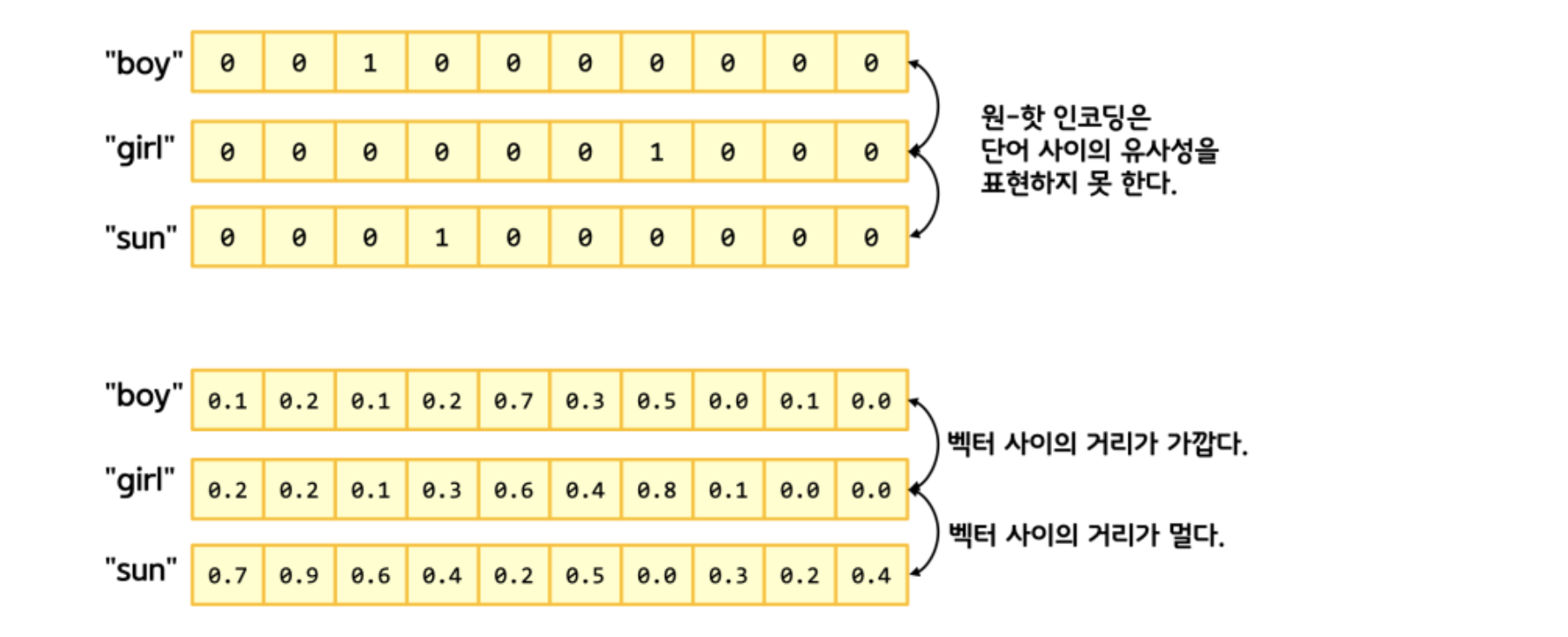
최적화를 위해서 원핫인코딩을 대체해서 관계를 표현하면 이것만으로 10%정도 정확도가 올라간다.
model_ebd = Sequential()

model_ebd.add(Embedding(1000, 32))
model_ebd.add(SimpleRNN(8))
model_ebd.add(Dense(1, activation=‘sigmoid’))

model_ebd.summary()
RNN은 앞뒤로 연관이 되어있기 때문에 거리가 멀면 학습이 어려워지는 문제가 있다. 그래서 tanh로는 한계가 있고, LSTM(Long short-term memory) 구조를 사용한다고 한다.
model.add(tf.keras.layers.LSTM(units=64))
뭐 역시나 Keras에서의 적용은 어렵지않다.
전반적으로 CNN보다 훨씬 어려운 것 같다. 그래서 개념적으로만 정리했고, 앞으로는 더 어려운 CAM 그리고 더 어려운 GAN(Generative Adversarial Network)같은 적대적 신경망같은 세계도 있다. 갈길은 먼데 계속 갈지는 모르겠다.